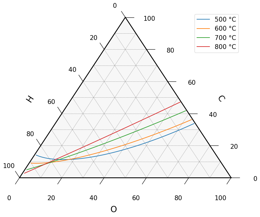
Carbon Deposition in a C-H-O Ternary Diagram

This example calculates the carbon deposition boundaries for gas mixtures of the elements carbon, hydrogen and oxygen and shows them in a ternary diagram. On the carbon-rich side of a boundary the formation of solid carbon is thermodynamically favored.

import gaspype as gp
import numpy as np
import matplotlib.pyplot as plt
import ternary

Setting temperatures and pressure. The temperatures get an additional dimension, so they are broadcast against the compositions later on:

t_range = np.array([500, 600, 700, 800])  # °C
t = t_range[:, None] + 273.15  # K

p = 1e5  # Pa

The search for the boundaries below runs through arbitrary atomic compositions. Oxygen (O2) and atomic carbon gas (C) are part of the fluid system to make sure that an equilibrium composition exists for each of them, also with an excess of oxygen or carbon:

fs = gp.fluid_system(['H2', 'H2O', 'CO2', 'CO', 'CH4', 'O2', 'C'])

The mixtures are defined by their atomic composition. Therefore we create an elements object with one mol of atoms for each of the three elements:

carbon = gp.elements({'C': 1}, fs)
hydrogen = gp.elements({'H': 1}, fs)
oxygen = gp.elements({'O': 1}, fs)

Each mixture is described by its molar fraction of carbon xc and by the hydrogen fraction of the remaining atoms h_ratio = H / (H + O). The following function returns the molar fractions of hydrogen and oxygen:

h_ratio = np.linspace(0.01, 0.99, 50)


def get_h_o_fractions(xc):
    xh = (1 - xc) * h_ratio
    xo = 1 - xc - xh
    return xh, xo

gp.carbon_activity calculates the activity of solid carbon (graphite) for the equilibrium state of a mixture. The shapes of the mixture, the temperature and the pressure are broadcast against each other, so a single call returns the activities of all compositions for all temperatures:

def get_carbon_activity(xc):
    xh, xo = get_h_o_fractions(xc)
    mix = carbon * xc + hydrogen * xh + oxygen * xo
    return gp.carbon_activity(mix, t, p)

At the carbon deposition boundary the carbon activity is 1. For each hydrogen ratio and each temperature the carbon fraction of the boundary is searched by bisection: The carbon fraction is increased if the activity is below 1 and decreased otherwise, while the step size is halved with every iteration. All boundaries are searched at once:

xc = np.full((len(t_range), len(h_ratio)), 0.5)
step_size = 0.5

while step_size > 1e-5:
    activity = get_carbon_activity(xc)

    step_size /= 2
    xc = np.where(activity < 1, xc + step_size, xc - step_size)

activity = get_carbon_activity(xc)
xh, xo = get_h_o_fractions(xc)

A search has only found a boundary if its activity ended up close to 1. The other points are discarded:

on_boundary = (activity > 0.9) & (activity < 1.1)

Plot the carbon deposition boundaries. The points of the ternary diagram are tuples of the coordinates for the bottom, the right and the left axis in percent:

scale = 100
fig, ax = plt.subplots(figsize=(10, 8))
tax = ternary.TernaryAxesSubplot(ax=ax, scale=scale)

# Draw boundary and gridlines
tax.boundary(linewidth=2.0)
tax.gridlines(color="black", multiple=10)

tax.left_axis_label("H", fontsize=20, offset=0.2)
tax.right_axis_label("C", fontsize=20, offset=0.2)
tax.bottom_axis_label("O", fontsize=20, offset=0.2)

# Set ticks
tax.ticks(ticks=list(range(0, 110, 20)), axis='lbr', linewidth=1, fontsize=15, offset=0.04)

# Remove default matplotlib ticks and box
tax.clear_matplotlib_ticks()
tax.get_axes().axis('off')

for i, tc in enumerate(t_range):
    mask = on_boundary[i]
    plot_data = list(zip(xo[i, mask] * scale, xc[i, mask] * scale, xh[i, mask] * scale))
    tax.plot(plot_data, label=f'{tc} °C')

tax.legend(fontsize=15)

# The axis labels are only drawn by tax.show() or by this call
tax._redraw_labels()